The Real Cost of Gradient Accumulation on T4 and L4

Gradient accumulation exists to solve a memory problem. When an effective batch of 32 will not fit on a 16 GB T4, you cut it into micro-batches, accumulate the gradients, and the optimizer still sees the average it would have seen in a single pass. Most tutorials end the story there. They should not, because the split you choose changes wall-clock time even though the math stays identical, and on rented GPUs that difference is billed by the hour.

A community benchmark posted to Reddit shows how large the gap gets. Its author fine-tuned Qwen3-1.7B with LoRA through TRL for exactly 100 optimizer updates, holding model, data, sequence length, precision, and seed fixed, then compared three splits of the same effective batch of 4 on a T4 and an L4. Notation for the rest of this article: m×k means micro-batch size m with k gradient accumulation steps, so 1×4 is four micro-steps of one sample, and 4×1 is one batch of four samples with no accumulation.

GPU, 100 optimizer updates	1×4	2×2	4×1
T4	287.6 s	258.8 s	238.2 s
L4	213.0 s	119.5 s	124.8 s

Three details matter. Moving from 1×4 to 4×1 cut the T4 run by about 17 percent. The same move cut the L4 run by more than 40 percent. And on the L4, 2×2 actually beat 4×1, which means the fastest configuration is not always the largest micro-batch. Same model, same data, same optimizer step count, and a 1.8× spread between the slowest and fastest split on the L4 (about 1.2× on the T4).

That spread comes from three mechanical costs the gradient-equivalence math never models: fixed per-micro-step overhead, weight traffic that scales with the number of micro-steps, and tensor-core underutilization at small micro-batch. Because the T4 and L4 sit near memory-bandwidth parity while differing sharply in tensor compute, the size of the penalty depends on the micro-batch itself. The fastest configuration is therefore an empirical property of your exact GPU, model, and sequence mix. What follows decomposes the cost, explains why the two GPUs diverge so differently, and gives you a benchmark protocol that settles the question on your own stack in minutes.

What Gradient Accumulation Preserves, and What It Does Not

Accumulating k micro-batches of size m reproduces a single batch of m×k samples for the optimizer under one condition: each micro-batch loss must be divided by k before backward. Trainers typically compute a mean loss over the micro-batch, so backward yields the gradient of that mean. Accumulate four of those without dividing and you have summed four means, which is 4× the gradient a true batch of four would have produced. The optimizer cannot distinguish a steeper loss surface from a learning rate that silently quadrupled. This divide-loss-by-k pitfall is the classic trap of manual gradient accumulation, and a long-running PyTorch discussion of accumulation walks through the scaling in detail. Frameworks apply it for you when configured correctly; the Accelerate accumulation guide shows the same pattern in the Accelerate API.

Equivalence is also narrower than it looks. Even with correct scaling, a 1×4 run and a 4×1 run differ in dropout mask draws, in padding when sequence bucketing shifts, and in floating-point summation order across smaller reduction kernels. The gradients agree to within numerical noise; the execution shape does not. So the question "does micro-batch size affect training speed" splits cleanly in two: it leaves the optimization trajectory nearly untouched while changing GPU throughput materially. Effective batch size is a math decision; micro-batch is a machinery decision.

One elimination before dissecting the clock: the optimizer and scheduler run once per accumulation cycle in every split, so their cost per optimizer update is constant across 1×4, 2×2, and 4×1. The community benchmark observed exactly this, with optimizer time nearly flat while forward and backward regions carried the entire difference. Whatever explains the spread, it lives inside the micro-steps.

Where the Extra Time Goes in Every Micro-Step

Per-micro-step time decomposes into three rough terms: fixed overhead (kernel launches, host synchronization, Python glue), memory traffic (weights, activations, and gradients moving between HBM and the streaming multiprocessors), and useful compute. At a fixed effective batch, going from k=1 to k=4 leaves total compute nearly unchanged but multiplies the number of times you pay the first two terms.

The bandwidth floor

Start with the bandwidth term, because it dominates. A 7B model in FP16 occupies about 14 GB of weights. Reading those weights once from HBM at roughly 300 GB/s, the class of bandwidth both of these cards deliver, takes about 47 ms before a single unit of useful math. Forward needs the weights once; backward needs them again to route gradients through every frozen layer. That puts a floor near 0.1 s per micro-step on weight traffic alone, and k=4 accumulation steps means paying close to that floor four times. Same tokens, same math, nearly 4× the weight bytes. This is the cleanest one-line answer to why gradient accumulation is slower than one large batch: the compute is shared across the effective batch, the bytes are not.

Overhead that stops hiding

Each micro-step launches a full transformer forward and backward, easily hundreds of CUDA kernels. Measured kernel launch latencies put a single launch in the range of a few microseconds on typical systems, so the launch bill alone can reach a millisecond or two per micro-step, and it compounds across 100 optimizer updates. The deeper problem is exposure. With a large micro-batch, each kernel runs long enough that the host queues work far ahead and launch cost hides behind execution. At m=1 the kernels are so short that the GPU can drain the queue faster than the host fills it, and gaps open between kernels. The arithmetic intensity view, the ratio of math to bytes moved, is the right mental model: low intensity means short, bandwidth-limited kernels with exposed overhead, and m=1 LoRA passes sit squarely in that regime.

Why the T4 and L4 Diverge as the Micro-Batch Grows

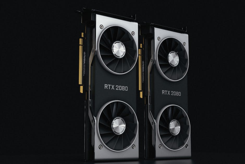
The datasheets explain the divergence pattern. Per NVIDIA's T4 datasheet, the Turing card carries 16 GB of GDDR6 at 320 GB/s and 65 dense FP16 TFLOPS. Per the L4 datasheet, the Ada card carries 24 GB at 300 GB/s and roughly 121 dense FP16 TFLOPS, plus BF16 and FP8 tensor paths. The Turing architecture whitepaper introduced FP16 and INT8 tensor cores without BF16; Ada, as covered in this Ada Lovelace overview, adds BF16 and FP8 throughput that Turing simply lacks.

Spec, per NVIDIA datasheets	T4 (Turing)	L4 (Ada)
Memory capacity	16 GB GDDR6	24 GB GDDR6
Memory bandwidth	320 GB/s	300 GB/s
Dense FP16 tensor throughput	65 TFLOPS	about 121 TFLOPS
BF16 and FP8 tensor paths	absent	present

The counterintuitive result falls out of this table. At m=1, both cards spend their time streaming the same weight bytes at nearly the same rate, so their times converge; in the community table the L4 finished 1×4 only about 26 percent ahead of the T4, with its doubled tensor throughput sitting largely idle. Grow the micro-batch and arithmetic intensity rises, because one weight read now feeds four rows of math. Compute takes a larger share of each step, the L4's tensor advantage engages, and the gap widens to roughly half the T4's wall-clock at 2×2 and 4×1. Capacity moves the finish line too: a 24 GB L4 can fit 4×1 with long sequences where a 16 GB T4 runs out of memory, so VRAM often decides whether a configuration is runnable before speed even enters the comparison.

The 2×2-beats-4×1 anomaly on the L4 is a reminder, not a contradiction. Tiling, cache behavior, and scheduler interactions make performance non-monotonic in micro-batch size, which is exactly why T4 vs L4 fine-tuning throughput has no single answer. It has a per-micro-batch answer, and only a timing run gives you that.

LoRA Shrinks the Optimizer, Not the Bandwidth Bill

A common misconception says adapter training makes micro-batch choice moot. The original LoRA paper freezes the base weights and trains small low-rank matrices per adapted module, and PEFT's LoRA reference documents the resulting collapse in trainable parameters, on the order of thousands of times fewer on large models. Optimizer state and gradient buffers shrink accordingly, which is why 7B fine-tuning fits on 16 GB at all.

The memory win does not touch the per-micro-step bandwidth bill. Every forward pass still reads all 7B base weights to produce activations, and every backward pass still reads them to route gradients into the adapters. The optimizer sees a tiny invoice; HBM sees the full one. The m×k asymmetry therefore survives LoRA intact: k accumulation steps still means roughly k full traversals of the frozen weights.

QLoRA changes the mix again. The QLoRA paper stores base weights in 4-bit and dequantizes them on the fly, fitting 65B fine-tuning on a single 48 GB GPU, at the price of extra quantization and dequantization kernels in every step. Gradient checkpointing trades the other direction, recomputing activations during backward to cut activation memory in exchange for more compute. Every knob here changes what fits in VRAM; none of them repeals the bandwidth floor. LoRA fine-tuning speed is still governed by how often you stream frozen weights.

A Repeatable Gradient Accumulation Benchmark

The way to benchmark gradient accumulation configurations is to hold everything constant except the split. The protocol:

1. Fix the run. Same seed, same dataset slice, same sequence-length mix, same precision. Every configuration must process the same total tokens.
2. Fix the work unit. Exactly 100 optimizer updates per configuration, then measure GPU training time per optimizer step by dividing the timed window by 100.
3. Exclude warmup. Run about 10 untimed updates first; clocks, caches, and memory allocators need to settle.
4. Synchronize around timing. Pair time.perf_counter with torch.cuda.synchronize. Unsynced timing measures the launch queue, not the GPU.
5. Take the median of three repeats. Rented GPUs throttle, and single runs lie.
6. Record torch.cuda.max_memory_allocated, reset between configurations. The OOM boundary is a finding, not a failure.
7. Sweep m upward until OOM, then report samples or tokens per second so numbers are comparable across splits.

A timing harness sketch

import statistics
import time
import torch

def bench(run_micro_step, reset_run, micro_bs, accum,
          updates=100, warmup=10, repeats=3):
    """Median seconds for `updates` optimizer steps, plus peak GB."""
    times = []
    for _ in range(repeats):
        reset_run(seed=1234)                   # same weights, same data order
        torch.cuda.reset_peak_memory_stats()
        for i in range((warmup + updates) * accum):
            if i == warmup * accum:
                torch.cuda.synchronize()       # timing starts after warmup
                start = time.perf_counter()
            run_micro_step(micro_bs, accum)    # one micro-step of the split
        torch.cuda.synchronize()               # drain the queue before stopping
        times.append(time.perf_counter() - start)
    peak_gb = torch.cuda.max_memory_allocated() / 1e9
    return statistics.median(times), peak_gb

Expect three patterns in your sweep. Times fall as m grows while the job is bandwidth-bound, then flatten or wobble as it turns compute-bound. Peak memory rises with m, mostly from activations. And the winner may be 2×2 rather than 4×1, as the L4 result showed, so test neighbors of your default rather than the endpoints alone.

Converting Timings Into Dollars per Fine-Tune

Cost per configuration equals measured seconds times the hourly rate divided by 3600. Two consequences follow.

First, the benchmark pays for itself immediately. If your sweep lands anywhere in the 17 to 44 percent range the community run showed, a two-hour job saves roughly 20 to 53 minutes of GPU time. The benchmark itself costs a handful of GPU-minutes, once.

Second, cross-GPU comparisons need the rate, not the name. A card wins whenever its rate-to-time product is the lowest, which makes the break-even pure arithmetic. Express the slowdown as a time ratio and invert it. A T4 that needs 1.4× the L4's wall-clock still wins as long as its hourly rate is at least 29 percent lower, because 1/1.4 = 0.71. A T4 that needs 1.8×, the size of the L4's own 1×4-versus-2×2 gap, needs a rate at least 44 percent lower, because 1/1.8 = 0.56. The cheaper card per hour is not automatically the cheaper fine-tune, and neither is the faster one. Check current GPU rental prices for your provider and multiply, and redo the lookup whenever rates move. Dollars per fine-tune picks the winner, and it is the only metric that survives contact with an invoice.

Failure Modes and Decision Rules

Most of what can go wrong in a short benchmark is already handled by the protocol itself: synchronize around timing, exclude warmup, take medians, record peak memory. The traps that survive a clean protocol are subtler, and both can corrupt a table like the community one.

• Dynamic padding quietly changes the work between splits. At m=1 each micro-batch pads to its own sequence; at m=4 it pads to the longest of four. Unless bucketing is fixed, your 1×4 and 4×1 runs process different token counts, so part of the measured spread is padding arithmetic, not accumulation mechanics. A padding shift of a few percent could fake or erase a micro-batch effect the size of the T4's 17 percent gap.

• Comparing splits with different effective batch sizes answers an optimization question, not a throughput one. The community table is only readable because 1×4, 2×2, and 4×1 all sum to the same effective batch of 4. Pit 4×1 against 2×4 and any speed difference is confounded with a different gradient estimate and half as many optimizer updates over the same data.

The rest is one line: judge speed by wall-clock and tokens per second, never the loss curve, and check nvidia-smi clocks if medians drift.

The decision rules that come out of all of this:

1. Start from the largest micro-batch that fits with headroom for your longest sequences.
2. Benchmark 1×k, the halving in the middle, and m×1, then pick the median-fastest rather than the single best run.
3. Expect diminishing returns from m=2 to m=4 as the job shifts toward compute-bound, and occasional reversals beyond that.
4. Keep accumulation when memory forces it, or when you need a large effective batch on a small GPU. It is the right tool, just not a free one.

Tell a colleague this: effective batch size chooses the math, micro-batch chooses the machinery, and machinery answers only to a stopwatch.