Why Speculative Decoding Pays Nearly 4x on CPUs

A server CPU decoding one token at a time is mostly empty silicon. Every token forces a full pass over the model's weights, so the memory system runs near its limit while the arithmetic units, and most of the cores, barely wake up. Speculative decoding is the trade that closes that gap: it spends the idle compute to verify several drafted tokens per weight read. The recently reported DFlash result, 3.92x autoregressive throughput on Intel Xeon 6 at concurrency 1, is a nearly 4x gain, and it is what the trick looks like on hardware with headroom to burn.

This article does the arithmetic behind that number, shows how much of it you should actually expect, explains when the gain evaporates, and works out when CPU LLM inference beats a rented GPU or a hosted API on cost per token.

The 3.92x Result and What It Measures

The number making the rounds comes from benchmark testing of DFlash, a CPU-focused inference engine built around draft-model speculation, described in coverage of Databricks' push to speed up open-source LLMs on CPUs (Databricks' Flash announcement). As reported, DFlash delivered 3.92x the autoregressive throughput with a Qwen3.5-9B model on Intel Xeon 6, in vLLM-based tests, at concurrency 1.

Every clause of that sentence matters:

• Single stream. One request, one sequence of tokens. This is the regime of an agent loop, a local dev REPL, or a single-stream batch job, not multi-tenant serving.
• Throughput, not quality. The method is distribution-preserving (more below), so the gain is speed, not a trade against accuracy.
• Decode, not prefill. The measurement is about generating tokens, and prefill for long prompts is a different, compute-heavy regime.

What the benchmark does not tell you is equally important: how the gain behaves with five concurrent agent sessions, what the acceptance rate was on different task types, or what the cost picture looks like against alternatives. Those are the three open questions this article closes, starting with why the trick works at all.

Why Single-Stream Decode Is Memory-Bandwidth-Bound

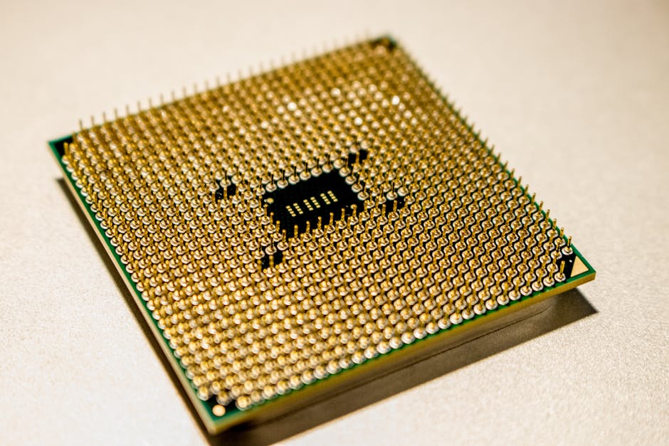
At batch size 1, generating one token means reading essentially every weight in the model once. The arithmetic per token is almost an afterthought. Walk the numbers for a 9B model quantized to int8 on a server-class machine, with assumptions labeled so you can substitute your own:

weights per token    9B params x 1 byte (int8)    ~= 9 GB
bandwidth ceiling    300 GB/s effective DRAM      ~= 33 tokens/s ceiling
compute per token    ~2 FLOPs x 9B params         ~= 18 GFLOPs
compute actually     33 tokens/s x 18 GFLOPs      ~= 0.6 TFLOP/s

A large Xeon socket delivers orders of magnitude more compute than 0.6 TFLOP/s, so at single-stream the arithmetic units sit mostly idle while memory bandwidth is the binding constraint. The arithmetic intensity here is roughly 2 FLOPs per byte, far below the balance point of any modern accelerator. This is the standard roofline argument for token generation, worked through in detail in this transformer inference arithmetic primer.

Two refinements matter for CPUs specifically. First, the ceiling is set by DRAM bandwidth, which is why Intel keeps pushing channels and faster modules; the platform's Xeon 6 MRDIMM brief exists precisely because workloads like this live and die by sustained bandwidth. Second, long contexts add KV-cache reads on top of the weight traffic, which squeezes the ceiling further.

The conclusion from the roofline: the budget is bytes per token, and compute is nearly free at batch 1. Any technique that buys more tokens per byte read wins, until it runs out of free compute.

How Draft and Verify Turns Idle Compute Into Tokens

Speculative decoding runs two models. A small draft model, often 10 to 20 times smaller than the target, proposes the next k tokens autoregressively. The target model then verifies all k candidates in a single forward pass, accepting the longest prefix it agrees with and resampling the first disputed position from its own distribution.

A concrete k=4 cycle:

1. The draft model proposes: The, cat, sat, on.
2. The target model scores all four positions in one pass.
3. It agrees with the first three and disagrees on the fourth.
4. Accept The cat sat, resample token four from the target's own distribution, and continue.

You emitted 4 tokens for one target pass plus four cheap draft passes. Because the verification pass computes all candidate positions at once, it reads the weights once for k tokens instead of once per token. The work shifts from matrix-vector products (one token per weight read) to matrix-matrix products (k tokens per weight read). FLOPs increase, but they were idle, and bandwidth does not.

The non-obvious part is that this is lossless by construction. The standard rejection-sampling acceptance rule provably preserves the target model's output distribution, established in Leviathan et al.'s paper and independently in Chen et al.'s speculative sampling. In expectation, the outputs are identical to running the target model alone. There is no quality knob being turned to buy speed.

Why Speculative Decoding Pays More on CPU Than GPU

The algorithm is identical on both architectures, yet the reported payoff differs. The original papers and most GPU results cluster around 2 to 3x at batch size 1, while this CPU result is nearly 4x. The gap is structural, not lucky.

Three mechanisms favor the CPU:

• A bigger idle fraction to harvest. A 64- to 128-core socket decoding one token at a time leaves most cores and most per-core matrix engines unused. A single-stream GEMV workload is close to the worst case for a wide CPU: no reuse across tokens, memory latency exposed, AMX tiles nearly empty. Batched verification suddenly fills those tiles and engages many cores at once.
• Cheap drafting. The small draft model fits comfortably in cache on a CPU, so the drafting overhead per cycle is low relative to the target pass.
• A less optimized baseline. Single-stream CPU decode has historically left more performance on the table than mature GPU kernels, so there is simply more to recover.

The honest framing: reported GPU gains of 2 to 3x and this CPU result of 3.92x are both the same arbitrage, amortizing one weight read across multiple tokens. The CPU just starts with proportionally more idle silicon to spend.

Acceptance Rate and Draft Length Decide Your Gain

How much of the 4x you keep is governed by one dominant variable: the per-token acceptance rate between draft and target, call it α. Under a simplifying independence assumption from the original analysis, the expected tokens emitted per verify step are:

E[tokens per step] = (1 − α^(k+1)) / (1 − α), where k is the number of drafted tokens.

Net speedup divides that by total step time (target pass plus draft passes). Assuming draft overhead of 25% of a target pass:

Per-token acceptance α	k=4, gross tokens/step	Net speedup (25% overhead)
0.3	1.43	1.14x, roughly break-even
0.5	1.94	1.55x
0.7	2.77	2.22x
0.9	4.10	3.28x

Two lessons fall out of the table. First, low acceptance can make speculative decoding slower than plain decoding, because you pay draft and verification costs for tokens you throw away. Second, draft length saturates: at α = 0.7, raising k from 4 to 8 adds roughly 0.4 expected tokens while doubling draft work, which is why optimal k is usually small, in the 3 to 6 range.

Acceptance rate is a property of your workload, not just your models. Structured output, code, and repetitive agent chatter tend to accept well because the next token is often predictable. Open-ended creative generation accepts poorly. Draft-target alignment matters too: same tokenizer and same model family, or a distilled draft, typically beats an arbitrary small model.

Before deploying, measure your own α: run a few hundred prompts with a draft enabled, log accepted-token counts per step, and plug the observed rate into the formula. Ten minutes of measurement replaces a week of hoping.

Why the Speedup Collapses at High Concurrency

Batching is the native amortizer of memory bandwidth. At concurrency C, the server already reads the weights once for roughly C tokens, so effective bytes per token fall by C and arithmetic intensity rises by the same factor. Speculation's advantage is that its extra FLOPs are free. As C grows, they stop being free and start competing for real compute, and the speculative decoding speedup trends toward 1x, sometimes below it once drafting overhead is counted.

The crossover is workload- and hardware-dependent, but the direction is certain and the erosion begins early, well before the machine saturates. This is why the DFlash number is explicitly a concurrency-1 result, and why you should read it as such: speculation buys latency, not aggregate throughput.

The practical routing follows directly. Single-stream or low-concurrency workloads, agent loops, local dev, sequential batch jobs, get the full benefit on CPU. A busy endpoint with dozens of concurrent requests is already amortizing its weight reads; adding speculation there mostly adds FLOPs.

CPU vs GPU vs API, a Cost per Token Framework

The deployment question reduces to one formula with honest inputs:

Cost per 1M tokens = hourly cost x 1,000,000 / (effective tokens per second x 3,600)

Plug in measured numbers, not vendor best cases. An illustrative low-concurrency setup, with list-price ballparks that vary by provider and region:

• CPU instance. A large CPU VM often rents in the low single digits per hour. At ~50 tok/s effective with speculation (a 9B int8 model starting in the teens, roughly 3x improved), that is ~180k tokens per hour, or roughly $11 per 1M tokens at $2/hr. On hardware you already own, the marginal cost approaches power and ops, which can push below hosted per-token pricing for frontier-class output. Utilization is the catch: the meter runs whether tokens flow or not.
• Rented GPU. Mid-tier GPUs rent around $1 to $3 per hour and H100-class from roughly $10 to $40+ on demand. A single stream uses a small fraction of that machine, so at concurrency 1 you are renting idle headroom. GPUs win decisively once batching fills them.
• Hosted API. You pay per token with zero idle cost and zero ops. Cheap open-model endpoints can undercut self-hosting on raw price; frontier endpoints cost far more per token but include the model you may actually need.

Option	Cost basis	Single-stream latency	Concurrency scaling	Best fit
CPU instance	Low hourly, meter runs always	Good with speculation	Poor past modest concurrency	Steady low-concurrency loops, owned boxes, data-locality needs
Rented GPU	Higher hourly	Fast	Strong with batching	Batch throughput, traffic spikes
Hosted API	Per token, no idle	Good	Elastic	Spiky volume, zero ops, no hardware

There is no universal crossover. Compute it per deployment: your acceptance-adjusted tokens per second, your effective hourly cost at your real utilization, and the API price for a model that meets your quality bar. The framework, not a magic threshold, is the deliverable.

Getting Started and When to Skip Speculation

The fastest path to a real number on your own hardware:

1. llama.cpp. Point it at a target model and a smaller draft model from the same family, tune the draft length, and compare tokens per second with and without. The llama.cpp speculative decoding docs cover the exact flags and supported configurations.
2. vLLM. Exposes speculative decoding through a draft-model configuration with a tunable speculative-token count, the same stack used in the DFlash testing.
3. DFlash. If you want the engine from the benchmark itself, track Databricks' releases rather than assuming the benchmark configuration transfers to your workload.

Use speculation when concurrency is 1 to a handful, output latency matters, generation is structured or repetitive, a same-family draft model exists, and the weights are quantized so bandwidth arithmetic favors you.

Skip it when you are serving many concurrent requests, generation is open-ended with low acceptance, you need aggregate throughput, or a GPU is already running hot.

The three questions from the opening now have answers. The 3.92x works because batch-1 decode is bandwidth-bound and verification converts idle CPU compute into extra tokens per weight read. Your realized gain is set by acceptance rate and draft length, and it can fall below break-even. The advantage dies as concurrency rises, because that is when compute stops being free. And on cost per token, CPU wins in the narrow but common case of steady low-concurrency work, especially on hardware you already run. Reproduce the arithmetic for your model, measure your acceptance rate, and the CPU-vs-GPU-vs-API decision becomes math instead of folklore.